社区微信群开通啦,扫一扫抢先加入社区官方微信群

社区微信群
从零开始学习神经网络
在说神经网络之前,我们讨论一下神经元(Neurons),它是神经网络的基本单元。神经元先获得输入,然后执行某些数学运算后,再产生一个输出。比如一个2输入神经元的例子: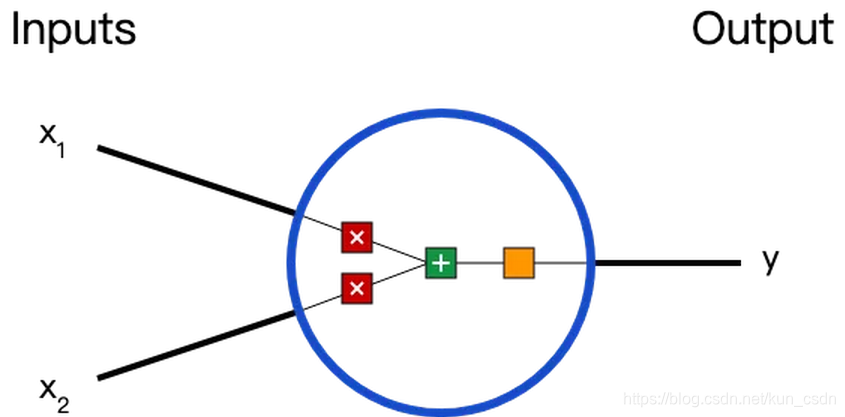
在这个神经元里,输入总共经历了3步数学运算,
先将输入乘以权重(weight):
最后经过激活函数(activation function)处理得到输出:
激活函数的作用是将无限制的输入转换为可预测形式的输出。一种常用的激活函数是sigmoid函数: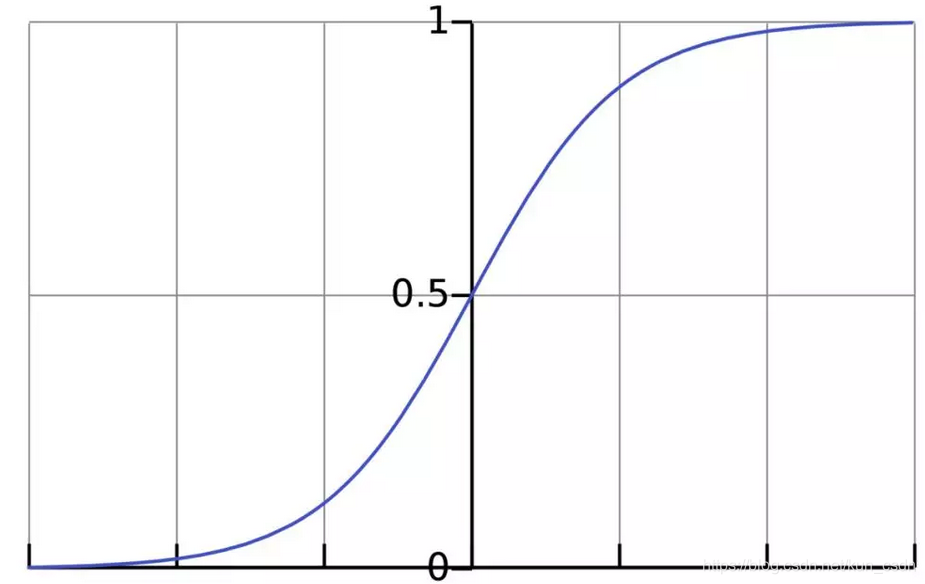
sigmoid函数的输出介于0和1,我们可以理解为它把 (−∞,+∞) 范围内的数压缩到 (0, 1)以内。正值越大输出越接近1,负向数值越大输出越接近0。
举个例子,上面神经元里的权重和偏置取如下数值:
是的向量形式写法。给神经元一个输入,可以用向量点积的形式把神经元的输出计算出来:
以上步骤的Python代码是:
import numpy as np

def sigmoid(x):
    # our activation function: f(x) = 1 / (1 * e^(-x))
    return 1 / (1 + np.exp(-x))

class Neuron():
    def __init__(self, weights, bias):
        self.weights = weights
        self.bias = bias

    def feedforward(self, inputs):
        # weight inputs, add bias, then use the activation function
        total = np.dot(self.weights, inputs) + self.bias
        return sigmoid(total)

weights = np.array([0, 1]) # w1 = 0, w2 = 1
bias = 4
n = Neuron(weights, bias)

# inputs
x = np.array([2, 3])   # x1 = 2, x2 = 3
print(n.feedforward(x)) # 0.9990889488055994
神经网络就是把一堆神经元连接在一起,下面是一个神经网络的简单举例:
这个网络有2个输入、一个包含2个神经元的隐藏层(h1和h2)、包含1个神经元的输出层o1。
隐藏层是夹在输入输入层和输出层之间的部分,一个神经网络可以有多个隐藏层。
把神经元的输入向前传递获得输出的过程称为前馈(feedforward)。
我们假设上面的网络里所有神经元都具有相同的权重和偏置,激活函数都是,那么我们会得到什么输出呢?
以下是实现代码:
class OurNeuralNetworks():
    """
    A neural network with:
      - 2 inputs
      - a hidden layer with 2 neurons (h1, h2)
      - an output layer with 1 neuron (o1)
    Each neural has the same weights and bias:
      - w = [0, 1]
      - b = 0
    """
    def __init__(self):
        weights = np.array([0, 1])
        bias = 0

        # The Neuron class here is from the previous section
        self.h1 = Neuron(weights, bias)
        self.h2 = Neuron(weights, bias)
        self.o1 = Neuron(weights, bias)

    def feedforward(self, x):
        out_h1 = self.h1.feedforward(x)
        out_h2 = self.h2.feedforward(x)

        # The inputs for o1 are the outputs from h1 and h2
        out_o1 = self.o1.feedforward(np.array([out_h1, out_h2]))
        return out_o1

network = OurNeuralNetworks()
x = np.array([2, 3])
print(network.feedforward(x)) # 0.7216325609518421
现在我们已经学会了如何搭建神经网络,现在再来学习如何训练它,其实这是一个优化的过程。
假设有一个数据集,包含4个人的身高、体重和性别:
| Name | Weight (lb) | Height (in) | Gender |
|---|---|---|---|
| Alice | 133 | 65 | F |
| Bob | 160 | 72 | M |
| Charlie | 152 | 70 | M |
| Diana | 120 | 60 | F |
现在我们的目标是训练一个网络,根据体重和身高来推测某人的性别。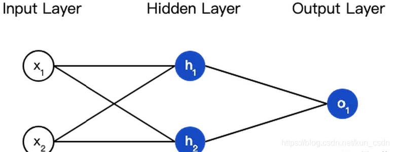
为了简便起见,我们将每个人的身高、体重减去一个固定数值,把性别男定义为1、性别女定义为0。
| Name | Weight (减去135) | Height (减去66) | Gender |
|---|---|---|---|
| Alice | -2 | -1 | 0 |
| Bob | 25 | 6 | 1 |
| Charlie | 17 | 4 | 1 |
| Diana | -15 | -6 | 0 |
在训练神经网络之前,我们需要有一个标准定义它到底好不好,以便我们进行改进,这就是损失(loss)。
比如用均方误差(MSE)来定义损失:
是样本的数量,在上面的数据集中是4;
代表人的性别,男性是1,女性是0;
是变量的真实值,是变量的预测值。
顾名思义,均方误差就是所有数据方差的平均值,我们不妨就把它定义为损失函数。预测结果越好,损失就越低,训练神经网络就是将损失最小化。
如果上面网络的输出一直是0,也就是预测所有人都是男性,那么损失是
| Name | |||
|---|---|---|---|
| Alice | 1 | 0 | 1 |
| Bob | 0 | 0 | 0 |
| Charlie | 0 | 0 | 0 |
| Diana | 1 | 0 | 1 |
如果觉得我的文章对您有用,请随意打赏。你的支持将鼓励我继续创作!
