在医学图像处理，尤其是在处理血管断层扫描类（如OCT、IVUS等）图像的过程中，不可避免的会使用到极坐标变换，也即是我们通常所说的“方转圆”。同样，我们可以使用极坐标变换的反变换实现“圆转方”

极坐标变换及其反变换的关键在于，根据极坐标变换前的图像（我们称为“方图”）确定极坐标变换后的图像（我们称为“圆图”）上每个像素点的像素值。也即是找到“圆图”和“方图”间几何坐标的对应关系。

1、极坐标变换（方转圆）

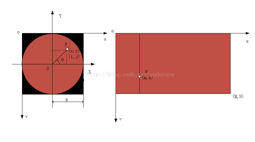
原理：如下图所示，实现极坐标变换的关键即在于找到圆图上任一点P(i,j)，在方图上对应的点p(m,n)，然后通过插值算法实现圆图上所有像素点的赋值。

方图上，其行列数分别为M、N，方图上的每一列对应为圆图上的每条半径，半径方向存在着一个长度缩放因子delta_r = M/R，圆周方向被分为N等分，即角度因子为delta_t = 2π/N；

圆图上，图像坐标（i,j）和世界坐标（x,y）有着如下变换关系：x = j - R, y = R - i；

那么，图中P点半径长度为r = sqrt(x*x + y*y)，角度theta = arctan(y/x)；

圆图上点P在方图上对应行数为r/delta_r；

圆图上点P在方图上对应的列数n = thata/delta_t。

以上就是极坐标变换的基本原理，结合相应的插值算法，即可实现图像的极坐标变换。

实现代码如下：

bool cartesian_to_polar(cv::Mat& mat_c, cv::Mat& mat_p, int img_d)
{
	mat_p = cv::Mat::zeros(img_d, img_d, CV_8UC1);

	int line_len = mat_c.rows;
	int line_num = mat_c.cols;

	double delta_r = (2.0*line_len) / (img_d - 1); //半径因子
	double delta_t = 2.0 * PI / line_num; //角度因子

	double center_x = (img_d - 1) / 2.0;
	double center_y = (img_d - 1) / 2.0;

	for (int i = 0; i < img_d; i++)
	{
		for (int j = 0; j < img_d; j++)
		{
			double rx = j - center_x; //图像坐标转世界坐标
			double ry = center_y - i; //图像坐标转世界坐标

			double r = std::sqrt(rx*rx + ry*ry);

			if (r <= (img_d - 1) / 2.0)
			{
				double ri = r * delta_r;
				int rf = (int)std::floor(ri);
				int rc = (int)std::ceil(ri);

				if (rf < 0)
				{
					rf = 0;
				}
				if (rc > (line_len - 1))
				{
					rc = line_len - 1;
				}

				double t = std::atan2(ry, rx);

				if (t < 0)
				{
					t = t + 2.0 * PI;
				}

				double ti = t / delta_t;
				int tf = (int)std::floor(ti);
				int tc = (int)std::ceil(ti);

				if (tf < 0)
				{
					tf = 0;
				}
				if (tc > (line_num - 1))
				{
					tc = line_num - 1;
				}

				mat_p.ptr<uchar>(i)[j] = interpolate_bilinear(mat_c, ri, rf, rc, ti, tf, tc);
			}
		}
	}

	return true;
}

顺便给一段双线性插值的代码：

uchar interpolate_bilinear(cv::Mat& mat_src, double ri, int rf, int rc, double ti, int tf, int tc)
{
	double inter_value = 0.0;

	if (rf == rc && tc == tf)
	{
		inter_value = mat_src.ptr<uchar>(rc)[tc];
	}
	else if (rf == rc)
	{
		inter_value = (ti - tf) * mat_src.ptr<uchar>(rf)[tc] + (tc - ti) * mat_src.ptr<uchar>(rf)[tf];
	}
	else if (tf == tc)
	{
		inter_value = (ri - rf) * mat_src.ptr<uchar>(rc)[tf] + (rc - ri) * mat_src.ptr<uchar>(rf)[tf];
	}
	else
	{
		double inter_r1 = (ti - tf) * mat_src.ptr<uchar>(rf)[tc] + (tc - ti) * mat_src.ptr<uchar>(rf)[tf];
		double inter_r2 = (ti - tf) * mat_src.ptr<uchar>(rc)[tc] + (tc - ti) * mat_src.ptr<uchar>(rc)[tf];

		inter_value = (ri - rf) * inter_r2 + (rc - ri) * inter_r1;
	}

	return (uchar)inter_value;
}

2、极坐标变换的反变换（圆转方）

原理：顾名思义，极坐标变换的反变换即极坐标变换的逆变换，原理和极坐标变换类似，只是更为直接和方便，且不需要进行插值，这里就不再赘述了。

直接看代码吧：

bool polar_to_cartesian(cv::Mat& mat_p, cv::Mat& mat_c, int rows_c, int cols_c)
{
	mat_c = cv::Mat::zeros(rows_c, cols_c, CV_8UC1);

	int polar_d = mat_p.cols;
	double polar_r = polar_d / 2.0; // 圆图半径

	double delta_r = polar_r / rows_c; //半径因子
	double delta_t = 2.0*PI / cols_c;  //角度因子

	double center_polar_x = (polar_d - 1) / 2.0;
	double center_polar_y = (polar_d - 1) / 2.0;

	for (int i = 0; i < cols_c; i++)
	{
		double theta_p = i * delta_t; //方图第i列在圆图对应线的角度
		double sin_theta = std::sin(theta_p);
		double cos_theta = std::cos(theta_p);

		for (int j = 0; j < rows_c; j++)
		{
			double temp_r = j * delta_r; //方图第j行在圆图上对应的半径长度

			int polar_x = (int)(center_polar_x + temp_r * cos_theta);
			int polar_y = (int)(center_polar_y - temp_r * sin_theta);

			mat_c.ptr<uchar>(j)[i] = mat_p.ptr<uchar>(polar_y)[polar_x];
		}
	}
	return true;
}

3、结果

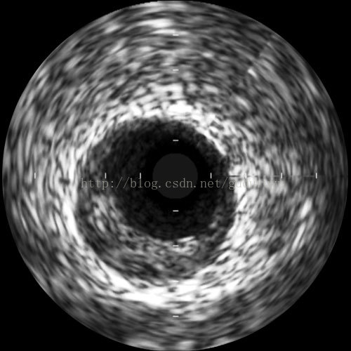
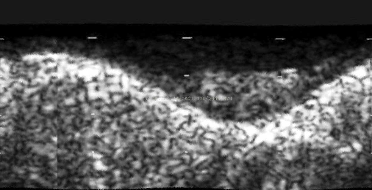
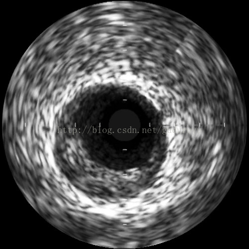
为验证算法，下载了一张IVUS(血管超声)图像，先用极坐标反变换得到方图，再用极坐标变换将方图变换回圆图，通过比较，变换前后的图像基本一致，哦了~~~

原始图

反极坐标变换图

极坐标变换结果

2017.03.24完成初稿