最近拿算法图解重新温习了一下算法，这本书真的非常适合入门，把比较简单算法细节和思路讲的非常清楚。

果然入门计算机语言就该学python。 大学里面一上来就C++太苦逼了。

        然后是第一次强烈的感受到Python解题的魅力。之前学python的时候，觉得不用定义就直接使用很变扭，还有就是可以灵活的使用各种数据结构，也是有点不适应。因为一开始学的就是C++，之前算法和数据结构都是用C++写的，后面工作用Java。Python还没拿来用过。某神说，leetcode里面排名考前的都是用python提交的，因为写起来跟伪代码差不多，有思路就好了，不用像c++、java那样考虑语言的特性。

        对于它们的语言特性最近的感受就是：Python就像塑料袋，什么东西都可以往里面塞，不怕变形，兼容性超好；Java像纸箱，类得写好了才能生成对象；C++跟java差不多，像木箱吧哈哈哈。

大概总结一下里面提到的算法吧：

一、算法简介

1.1二分查找 ：

一个有序数组中找一个数的位置（对应该数字所在数组下标index）。

def binary_search(list, item):
    low = 0
    high = len(list) - 1
    while low <= high:
        mid = int((low + high) / 2)
        guess = list[mid]
        if guess == item:
            return mid
        if guess > item:
            high = mid - 1
        else:
            low = mid + 1
    return None


my_list = [1, 3, 5, 7, 9]

print(binary_search(my_list, 3)) # => 1
print(binary_search(my_list, -1)) # => None

• 也可用递归实现
• 操作对象：数组
• 使用前提：有序的数组
• 性能方面：时间复杂度O(logn)

1.2 旅行商问题：

旅行商前往n个城市，确保旅程最短。求可能的排序：n!种可能。

 

二、选择排序

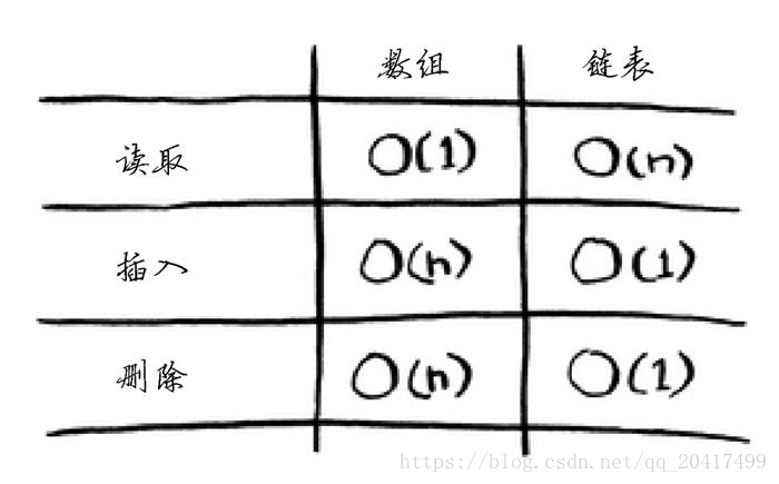
2.1 数组和链表

数组：连续存储在硬盘中；链表：分散存储在硬盘中；

 

2.2 选择排序：将数组元素按照从小到大的顺序排序，每次从数组中取出最小值

def findSmallest(arr):
    smallest = arr[0]
    smallest_index = 0
    for i in range(1, len(arr)):
        if arr[i] < smallest:
            smallest = arr[i]
            smallest_index = i
    return smallest_index

def selectionSort(arr):
    newArr = []
    for i in range(len(arr)):
        smallest = findSmallest(arr)
        newArr.append(arr.pop(smallest))
    return newArr


print(selectionSort([5, 3, 6, 2, 10])) #[2, 3, 5, 6, 10]

 

三、递归----一种优雅的问题解决方法

适用递归的算法要满足：

• 基限条件（即返回的条件）
• 递归条件（调用递归函数）

特点：

自己调用自己，调用栈在内存叠加，如果没有返回条件，将无限循环调用，占用大量内存，最终爆栈终止进程。

 

还有一种高级一点的递归：

尾递归 （将结果也放入函数参数，内存里面调用栈只有一个当前运行的函数进程）

举个简单的例子： 阶乘f(n) = n！

def fact(x):  #递归
    if x == 1:
        return 1
    else:
        return x * fact(x-1)  #注意这里跟尾递归不同


#尾递归
def factorial(x,result):  
    if x == 1:
        return result
    else:
        return factorial(x-1,x*result)


if __name__ == '__main__':
    print(fact(5)) #5*4*3*2*1 = 120
    print(factorial(5,1)) #120

 

四、快速排序 （分而治之策略）

• 每次选取数组中一个元素x当作分水岭（一般选取第一个元素）：[小于元素x的数组]+[x]+[大于元素x的数组]，然后递归调用，直到最后处理的数组元素只剩下零个或者一个
• 平均时间复杂度O(nlogn)
• 最差情况时间复杂度O(n^2)   (出现这个情况是：快排的数组本来就是有序的（顺序/倒序），选取的元素又是开头第一个的话，每次变成只能处理一侧的数组了。 改善：可以选取数组中间的元素当作分水岭pivot，只有两边的元素就都能均匀处理了)

#!/usr/bin/python

def quicksort(array):
    if len(array) < 2:
        return array
    else:
        pivot = array[0]
        less = [i for i in array[1:] if i <= pivot]  #超级像伪代码！
        print(less)
        greater = [i for i in array[1:] if i > pivot]
        print(greater)

    return quicksort(less) + [pivot] + quicksort(greater)
  

if __name__ == '__main__':
    print(quicksort([7,1,10,5,3,2,6]))

'''
[1, 5, 3, 2, 6]
[10]
[]
[5, 3, 2, 6]
[3, 2]
[6]
[2]
[]
[1, 2, 3, 5, 6, 7, 10]
'''

 

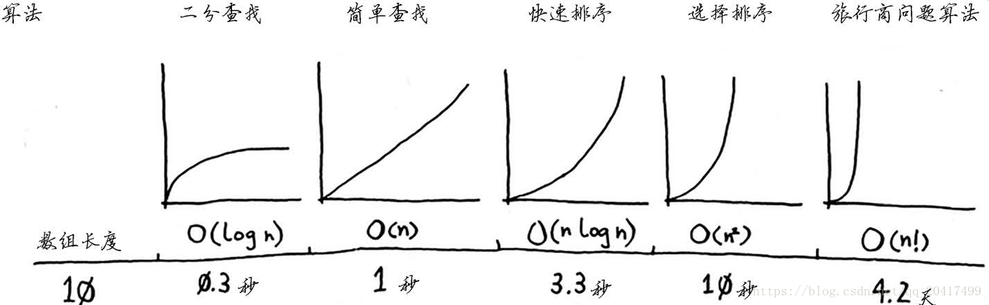
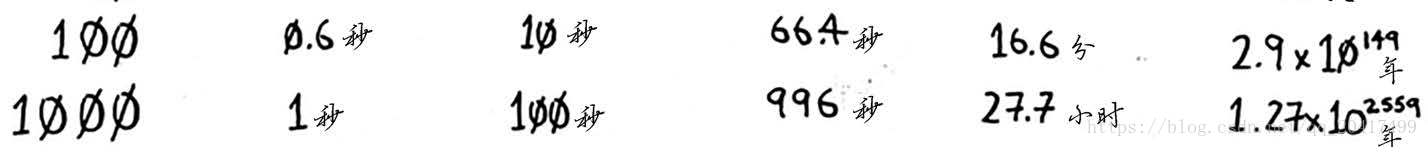
到目前算法为止，复杂度对比：

 

排序到算法有：

冒泡排序，选择排序，快速排序，归并排序，堆排序（感兴趣到小伙伴可以自己去搜索）

 

下面列出冒泡排序和归并排序算法：

#冒泡排序，每次寻找最小到元素往前排，就像汽水从下往上冒一样。所以叫冒泡排序啦
def simpleSort(array):
    for i in range(len(array)-1):
        for j in range(i,len(array)):
            if array[i] > array[j]:
                temp = array[i]
                array[i] = array[j]
                array[j] = temp
    return array


print(simpleSort([9,8,6,7,4,5,3,11,2])) #[2, 3, 4, 5, 6, 7, 8, 9, 11]


    

• 冒泡排序时间复杂度O(n^2)
• 两个for循环搞定，每一轮for循环找到一个最小值。for循环两两元素对比交换

 

归并排序：

def mergeSort(array):
    if len(array) < 2:
        return array
    else:
        mid = int(len(array)/2)
        left = mergeSort(array[:mid])
        right = mergeSort(array[mid:])
        return merge(left, right)

def merge(left, right): #并两个已排序好的列表，产生一个新的已排序好的列表
    result = []  # 新的已排序好的列表
    i = 0  # 下标
    j = 0
    # 对两个列表中的元素 两两对比
    # 将最小的元素，放到result中，并对当前列表下标加1
    while i < len(left) and j < len(right):
        if left[i] <= right[j]:
            result.append(left[i])
            i += 1
        else:
            result.append(right[j])
            j += 1
    # 此时left或者right其中一个已经添加完毕，剩下的就全部加到result后面即可      
    result += left[i:] 
    result += right[j:]
    return result

array = [9,5,3,0,6,2,7,1,4,8]
result = mergeSort(array)
print('排序后：',result) #排序后： [0, 1, 2, 3, 4, 5, 6, 7, 8, 9]

• 归并排序时间复杂度是O(nlogn)
• 最坏情况也是O(nlogn)
• 归并排序采用先分后总的方式，先按中间分，分到数组最后只有一个元素为止，最后两两合并。有点mapReduce的味道。

 

五、散列表（Hash）

散列函数： 散列函数是这样的函数，即无论你给它什么数据，它都还你一个数字。

模拟映射关系

散列（哈希）函数应用广泛：

• 快速查找
• 文件安全性传输交验
• 可以防止重复 （一旦发现重复，该哈希函数就不安全了。也就是说被破译了。）

•  缓存/ 记住数据，以免服务器再通过处理来生成它们。

性能：

•  散列表的填装因子 = （散列表包含的元素数）/（位置总数）
•  填装因子越低，发生冲突的可能性越小，散列表的性能越高。一个不错的经验规则是：一旦填装因子大于0.7 ，就调整散列表的长度。

良好的散列函数让数组中的值呈均匀分布。

糟糕的散列函数让值扎堆，导致大量的冲突。

 

六、广度优先搜索 （breadth-first search ，BFS ） 

 广度优先搜索是一种用于图的查找算法，可帮助回答两类问题：

第一类问题：从节点A 出发，有前往节点B 的路径吗？

 第二类问题：从节点A 出发，前往节点B 的哪条路径最短？

• 广搜采用双端队列
• 处理过程中，将所有有关的节点都添加到处理队列中
•  非加权图（无向图）中查找最短路径

看如下例子：从你的朋友关系网中，找出一个芒果销售商。（假设芒果销售商名字是以m结尾）

 

from collections import deque


#需编写函数person_is_seller，判断一个人是不是芒果销售商，如下所示。
def person_is_seller(name):
    return name[-1] == 'm' #这个函数检查人的姓名是否以m结尾：如果是，他就是芒果销售商。。


def bfs(graph,name):
    search_queue = deque()
    search_queue += graph[name]#graph["you"]是一个数组，其中包含你的所有邻居，如["alice", "bob","claire"]。这些邻居都将加入到搜索队列中。

    searched =[]
    while search_queue:
        person = search_queue.popleft()
        if not person in searched:
            if person_is_seller(person):
                print(person + " is a mango seller!")
                return True
            else:
                search_queue += graph[person]
                searched.append(person)
    return False


if __name__=='__main__':
    graph = {}
    graph["you"] = ["alice", "bob", "claire"]
    graph["bob"] = ["anuj", "peggy"]
    graph["alice"] = ["peggy"]
    graph["claire"] = ["thom", "jonny"  ]
    graph["anuj"] = []
    graph["peggy"] = [] 
    graph["thom"] = []
    graph["jonny"] = []

    print(graph)
'''
{'you': ['alice', 'bob', 'claire'], 
'bob': ['anuj', 'peggy'], 
'alice': ['peggy'], 
'claire': ['thom', 'jonny'], 
'anuj': [], 
'peggy': [], 
'thom': [], 
'jonny': []}
'''
    
    bfs(graph,"you")  #thom is a mango seller!

 

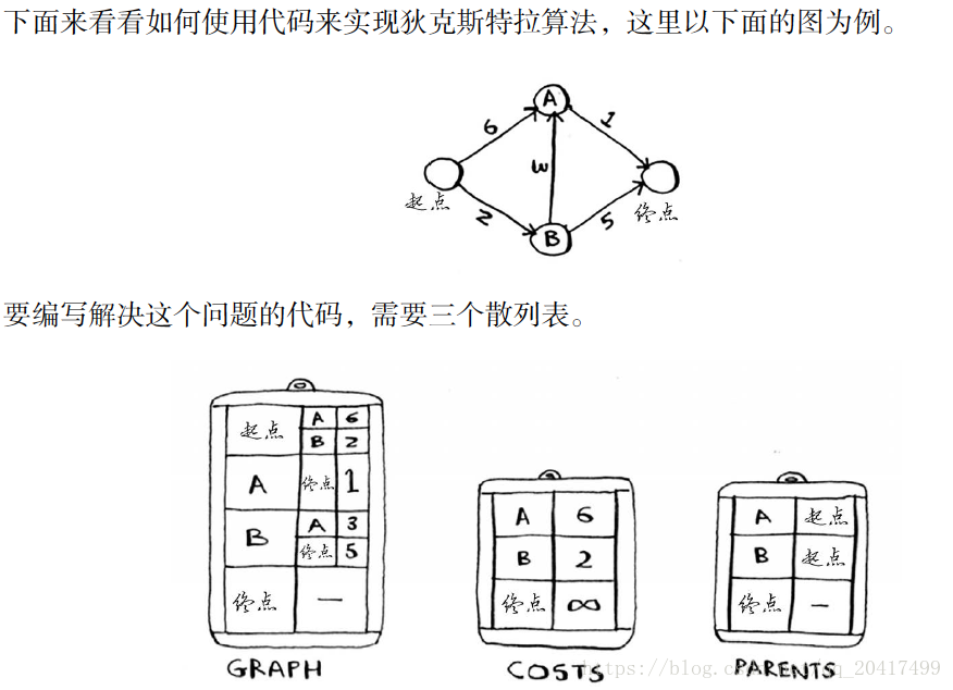
七、狄克斯特拉算法（ Dijkstra’s algorithm）

• 可以处理：有向无环图（directed acyclic graph，DAG）

•  加权图中查找最短路径

•  不能将狄克斯特拉算法用于包含负权边的图。在包含负权边的图中，要找出最短路径，可使用另一种算法—— 贝尔曼 福德算法（Bellman-Ford algorithm）

def find_lowest_cost_node(costs,processed):
    lowest_cost = float("inf")
    lowest_cost_node = None
    for node in costs:
        cost = costs[node]
        if cost < lowest_cost and node not in processed:
            lowest_cost = cost
            lowest_cost_node = node
    return lowest_cost_node

def dijkstra(graph,costs,parents):
    processed = []
    node = find_lowest_cost_node(costs,processed)
    while node is not None:
        cost=costs[node]
        neighbors=graph[node]
        for n in neighbors.keys():
            new_cost = cost + neighbors[n]
            if costs[n]>new_cost:
                costs[n]=new_cost
                parents[n]=node
        processed.append(node)
        node = find_lowest_cost_node(costs,processed)
    return costs,parents

if __name__ == '__main__':
     graph = {}
     graph["start"] = {}
     graph["start"]["a"] = 6
     graph["start"]["b"] = 6
     
     graph["a"] = {}
     graph["a"]["fin"] = 1

     graph["b"] = {}
     graph["b"]["a"] = 3
     graph["b"]["fin"] = 5

     graph["fin"] = {}


     infinity = float("inf")
     costs = {}
     costs["a"] = 6
     costs["b"] = 2
     costs["fin"] = infinity

     parents={}
     parents["a"]="start"
     parents["b"] = "start"
     parents["fin"] = None

     costs,parents = dijkstra(graph,costs,parents)
     print(costs) #{'a': 5, 'b': 2, 'fin': 6}
     print(parents) #{'a': 'b', 'b': 'start', 'fin': 'a'}
     
     
     

 

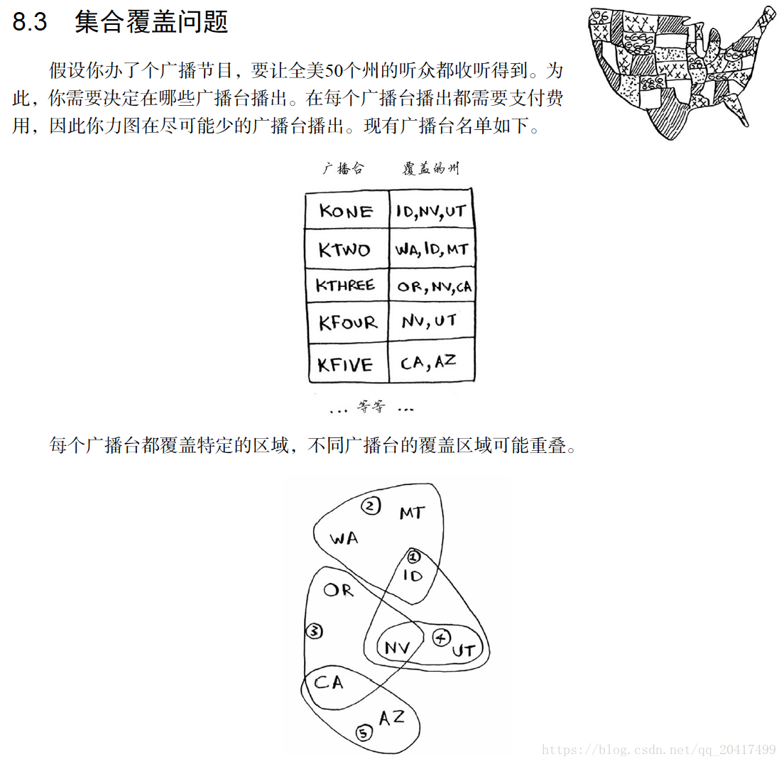
八、贪婪算法（贪心算法）

•  贪婪算法易于实现、运行速度快，是不错的近似算

•  贪婪算法寻找局部最优解，企图以这种方式获得全局最优解

 

可解决：

• 调度问题
• 背包问题
• 集合覆盖问题

stations = {}
stations["kone"] = set(["id", "nv", "ut"])
stations["ktwo"] = set(["wa", "id", "mt"])
stations["kthree"] = set(["or", "nv", "ca"])
stations["kfour"] = set(["nv", "ut"])
stations["kfive"] = set(["ca", "az"])
print(stations)
'''
{'kone': {'id', 'nv', 'ut'},
'ktwo': {'wa', 'mt', 'id'},
'kthree': {'ca', 'or', 'nv'},
'kfour': {'nv', 'ut'},
'kfive': {'ca', 'az'}}
'''

states_needed = set(['id', 'or', 'ut', 'wa', 'ca', 'az', 'nv', 'mt'])
print(states_needed)

final_stations = set()

while states_needed:
    best_station = None
    states_covered = set()
    for station, states in stations.items():
        covered = states_needed & states
        if len(covered) > len(states_covered):
            best_station = station
            states_covered = covered
    states_needed -= states_covered
    final_stations.add(best_station)

print(final_stations) #{'kfive', 'kthree', 'kone', 'ktwo'} 选择1235

 

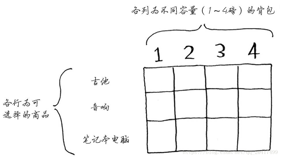
九、动态规划：将问题分成小问题，并先着手解决这些小问题

9.1动态规划，都可以画网格解决！

背包问题

 假设你是个小偷，背着一个可装4 磅东西的背包。

你可盗窃的商品有如下3 件：

音响，3000美元，4磅

笔记本电脑，2000美元，3磅

吉他，1500美元，1磅

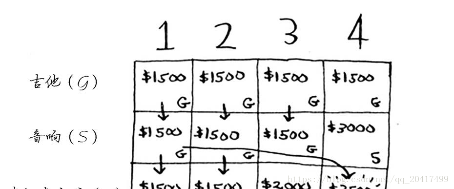
 每个动态规划算法都从一个网格开始，背包问题的网格如：

最终结果：

def bag(goods,size):
    cell = [[0 for col in range(size)] for row in range(len(goods))] 

    package_size= [i+1 for i in range(size)] 

    for j in range(size):
        if(goods[0][1]<=package_size[j]):
            cell[0][j] = goods[0][0]


    for i in range(1,len(goods)):
        for j in range(size):
            if (package_size[j]-goods[i][1]>0) and (goods[i][0] + cell[i-1][package_size[j]-1-goods[i][1]]) > cell[i-1][j]:
                cell[i][j] = goods[i][0] + cell[i-1][package_size[j]-goods[i][1]-1]
            elif (package_size[j]-goods[i][1]==0) and (goods[i][0] > cell[i-1][j]): 
                 cell[i][j] = goods[i][0]
            else:
                cell[i][j] = cell[i-1][j]
    print(cell)  #[[1500, 1500, 1500, 1500], [1500, 1500, 1500, 3000], [1500, 1500, 2000, 3500]]

    return cell[len(goods) - 1][size - 1]



if __name__ == '__main__':
    goods = [[1500,1],[3000,4],[2000,3]]
    print(bag(goods,4)) #3500

 动态规划功能强大，它能够解决子问题并使用这些答案来解决大问题。但仅当每个子问题都是离散的，即不依赖于其他子问题时，动态规划才管用。

最优解可能导致背包没装满。

 

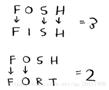
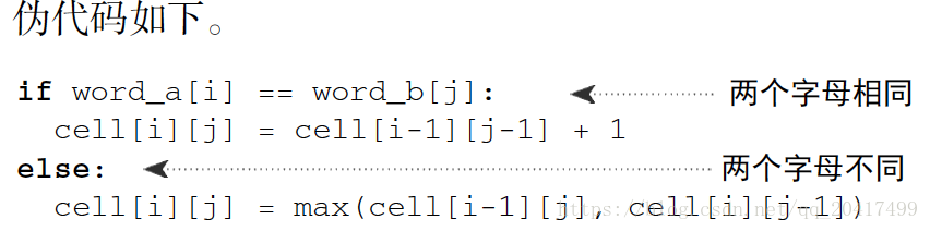
9.2 最长公共子串

 

9.3 最长公共子序列

 

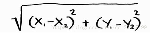
十、K最近邻算法（KNN）： KNN用于分类和回归，需要考虑最近的邻居

 要计算两点的距离，可使用毕达哥拉斯公式：

 KNN算法真的是很有用，堪称你进入神奇的机器学习领域的领路人！

 使用KNN 来做两项基本工作—— 分类和回归：

  分类就是编组；

  回归就是预测结果（如一个数字）

 特征抽取意味着将物品（如水果或用户）转换为一系列可比较的数字

 

 OCR指的是光学字符识别（ optical character recognition），这意味着你可拍摄印刷页面的照片，

计算机将自动识别出其中的文字。  一般而言，OCR 算法提取线段、点和曲线等特征

 

 垃圾邮件过滤器使用一种简单算法——朴素贝叶斯分类器 （Naive Bayes classifier ）

 朴素贝叶斯分类器能计算出邮件为垃圾邮件的概率，其应用领域与KNN 相似。

 

 

十一、其他算法

11.1 树

        二叉查找树： 平均访问时间也为O(log n）

 B树是一种特殊的二叉树，数据库常用它来存储数据

 如果你对数据库或高级数据结构感兴趣，请研究如下数据结构：B 树，红黑树，堆，伸展树。

11.2 反向索引：一个散列表，将单词映射到包含它的页面。这种数据结构被称为反向索引 （inverted index ），常用于创

建搜索引擎

11.3 傅立叶变换（分离数字信号，用sin+cos叠加）： 给定一首歌曲，傅里叶变换能够将其中的各种频率分离出来。

 

 与可扩展性和海量数据处理相关：

11.4并行算法（ 要改善性能和可扩展性，并行算法可能是不错的选择！）

11.5 MapReduce（ 分布式算法）

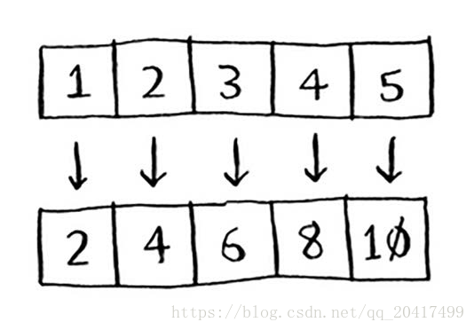
 映射（map ）函数和归并（reduce ）函数

 映射是将一个数组转换为另一个数组

 归并是将一个数组转换为一个元素

 

1.6 布隆过滤器和HyperLogLog

 

11.7 SHA 算法（ 散列函数是安全散列算法（secure hash algorithm ，SHA ）函数）

   给定一个字符串，SHA返回其散列值。

可用于比较文件/检查密码

 

11.8 局部敏感的散列算法

 有时候，你希望结果相反，即希望散列函数是局部敏感的。在这种情况下，可使用Simhash

 

11.9 Diffie-Hellman 密钥交换（ 公钥和私）

 Diffie-Hellman算法解决了如下两个问题：

 双方无需知道加密算法。他们不必会面协商要使用的加密算法。

 要破解加密的消息比登天还难。

 

11.10 线性规划 （初中知识。。常考题）

 目标是利润最大化，而约束条件是拥有的原材料数量。

 线性规划使用Simplex 算法， 这个算法很复杂（最优化）

 

 

 

欢迎关注本人微信公众号：